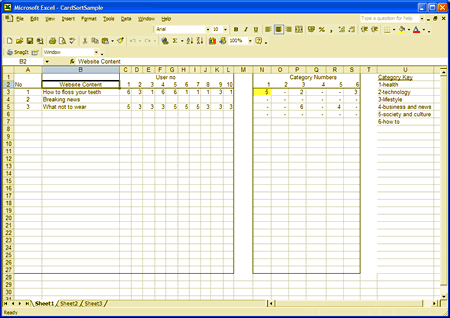
Following up from Digital Web Magazine and my card sort article, here is one way of analysing your results using a spreadsheet.
In the spreadsheet we need to set up two tables which will sit next to each other:
- Table 1 stores the number of users and their cards.
- Table 2 counts cards and identify patterns.
Download your own copy of the spreadsheet to tinker with at:
https://ruthstalkerfirth.com/CardSortSample.xls
or
https://ruthstalkerfirth.com/CardSortSample2024.xlsx (2024)
Table 1
Type the unique card identifier (number) in the first column, and the content description of each card in the second column; for example, Column A, ‘1’, Column B, ‘How to floss your teeth’. Then across the top, if you had ten pairs of users number the columns one to ten. As you go through each card sort from each user pair, type the number of the category they chose next to the description of the content. If user pair 3 put 1. How to floss your teeth under Category 6., How to, then you would type 6 in the column which represents user pair 3 next to content item 1. And, if user pair 4 put 1., How to floss your teeth under Category 1., Health, then you would type 1 in user pair 4’s column on content item 1’s row.
You may begin with only a few categories but as you work through the users solutions, you will see more user defined categories for which you need to create numbers. If you have several levels of categories, just carry on numerically naming the categories wherever they are in the hierarchy.
Table 2
On the same heading line as the user pairs’ numbers (in Table 1), create a row of column headers which represent the category heading numbers.
In each row of each column, we want to count the number of times the category heading appears in the user pair/content side of the spreadsheet. So, if we want to count up Category 1 Health in Table 1 we would put in that column on the first row (which because of our table headers is row 3) =COUNTIF($C3:$L3,1) and =COUNTIF($C3:$L3,1) on the second row, and so on. The C numbers should change down the column, but the second number after the comma which represents our Category 1 – should remain the same. The $ sign is used to lock the referring row otherwise copying the equation down the rows of the same column will cause the references to change. Table 2 will count up how many times you have a category. If the category appears many times you can highlight the count by changing the colour of the cell.
Keep typing
Entering data into a spreadsheet is boring and laborious. Be patient! Once all the data is in, it becomes much easier to get an insight into your users’ head. The interesting part begins.
As all statisticians know, if you torture the data enough, it will tell you anything.


5 comments
Comments are closed.